
By Katie Petrinec
For the past year, I’ve had the opportunity to really delve into our SWMP data with the goal of providing a 10-year analysis of SWMP data [almost] since the program’s inception at the GTMNERR. Analyses of the SWMP datasets are necessary to identify estuarine impacts of events like hurricanes or prolonged droughts, identify long-term trends, and address coastal management questions and issues. The goal of these analyses is to produce local, regional, or national summaries and reports.
A few years ago, we set-out with an objective to create a report that will provide a baseline of information on water quality and meteorological conditions in the GTM, for which future analyses can be built upon. Our SWMP program at the GTMNERR began in the early 2000’s with each component (water quality, nutrient, and weather) starting in different years. By 2003 we had the first complete dataset for each component! Naturally, we decided that the report should start there.
Where to begin?
The first step in putting together a report like this is to acquire the data and make sure it is in the right format to conduct the analysis. For those of you who use large datasets, you understand that preparing the data for analysis is no easy feat! Luckily, SWMP data (for all NERRS) is housed in one central location, appropriately named the Centralized Data Management Office (CDMO).
The CDMO has the responsibility of providing data management and access for SWMP data. If you are not familiar with SWMP data, it is important to know that it undergoes three levels of Quality Assurance/Quality Control (QA/QC) reviews. The first level (Primary QA/QC) is an automated assessment of data based on sensor limits and is conducted immediately upon submission of the raw (unedited) data file to the CDMO. A second level of QA/QC (Secondary QA/QC) is conducted by the reserve and results are submitted quarterly and annually to the CDMO. The final level of QA/QC (Tertiary QA/QC) occurs annually by the CDMO.
Interested in viewing or downloading our SWMP data? Visit www.nerrsdata.org!

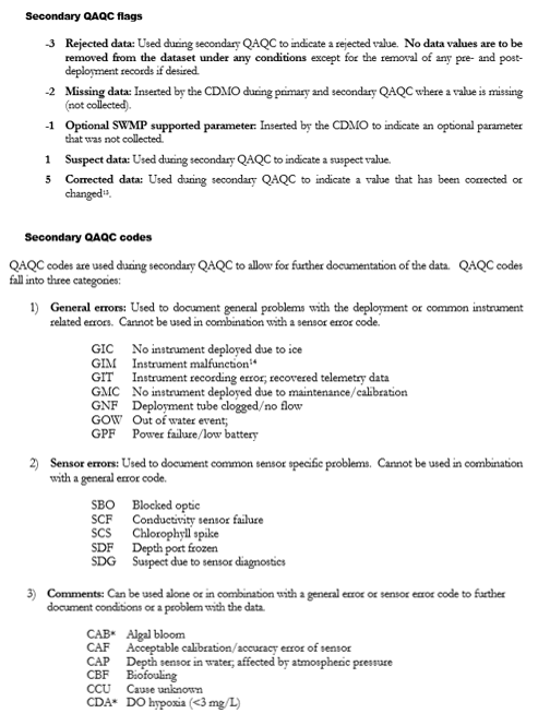
Most of 2015 was spent prepping the data files for analysis. After downloading the data files from the CDMO (2003 – 2012) you will notice that these files contain columns beginning with “F_”. These columns represent the ‘flag’ columns and provide information regarding the associated data value using a newly implemented standardized Secondary QAQC code. Huh?

Back in 2007, the CDMO enhanced the data submission process and provided new tools for NERR staff to analyze their SWMP data during the Secondary QA/QC process. Secondary QA/QC was implemented prior to 2007 but all documentation regarding the data was recorded in a metadata document. Therefore, physical codes were not assigned directly to values in the dataset. Data collected prior to 2007 (2006 through the onset of that NERRS SWMP program) was labeled as Historic. As such, the documentation of the data remained in these metadata documents, with no other specific codes in the data file except “Historic”.

What do we mean by “specific codes”?
Secondary QA/QC performed on data collected since 2007 are analyzed using macros in Microsoft Excel, which were created by the CDMO. These data files include a standardized coding method for the Secondary QA/QC reviews and all of these codes are explained in the metadata documents associated with each datafile.
After compiling 10-years of data (2003 – 2012) we made a few preliminary plots to visualize the data. We noticed that the differences in the data files-historic (pre-2007) and non-historic (2007-present)-made a difference in the analysis process. For example, we looked at a Turbidity plot containing data from 2002 – 2015 (exceeding our 10-year time frame) (Figure 5). While reviewing the plot, we realized that this data set includes a large amount of data that exceeds manufacturer sensor specifications. For our turbidity sensors, values that exceed 1000 NTUs are considered suspect/anomalous; meaning, “there is something strange going on here and you might not want to use these data in your analysis”. The sensor should not be reading that high.
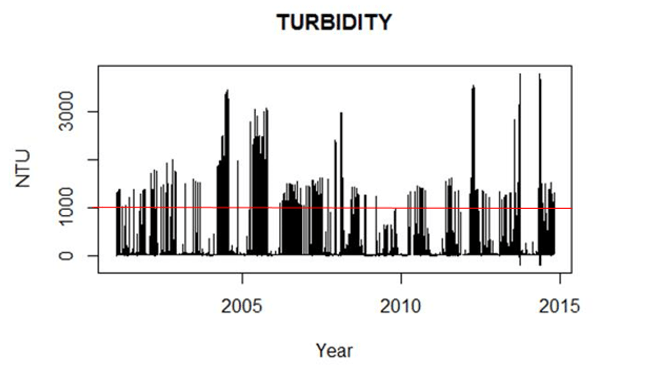
Sometimes we see things in (or on) our instruments that can give us clues as to why we might have such ‘spikes’ in turbidity values. One common culprit is a crab. They often get inside our instrument guards and stay there until we retrieve the instrument two weeks later. Sometimes, they even molt and grow too large to get back out of the guard through the mesh that surrounds it! While in the guard, every time the crab swims past the turbidity sensor optics, you can see a ‘spike’ in values-like the values that exceed 1000 NTUs (Figure 5). This type of information is explained in the metadata documents as we perform our Secondary QA/QC process. Today, we would code a value “ (CSM)”, indicating that this value is suspect and you should see our notes in the metadata where we explain that a crab had an adventure in our instrument.
After seeing that our dataset contained turbidity values that exceed 1000 NTUs. We realized that further steps were needed in preparing the data before we could begin any sort of analyses. If we were noticing these patterns in the turbidity data, what about the other parameters? It seems that the “Historic” coding was keeping all the data and not giving us the ability to select whether we wanted to include these “suspect/anomalous” values in our analysis.
Thus began the great task of re-coding files….
